How to Hide Data in a Worksheet in Excel

There may be times when you want to share or view some data in an Excel worksheet, but not all of its contents. In such cases, you can hide the data from view. In this Excel tutorial, I’ll show you two ways in which to hide data in a worksheet in Excel 2016.

Note: This method should not be used to hide sensitive information or hide protected information. The main purpose of this method of hiding data is to ensure that you avoid screen clutter and make the document more easy to read. Plus, its always nice to see a clean, professional looking worksheet, isn’t it?

There are actually 2 ways in which this can be accomplished. Let’s take a look at them.

How to Hide Data in a Worksheet : Method 1

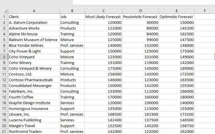
In our Forecasting Figures, let’s hide the Pessimistic and Optimistic revenue figures.

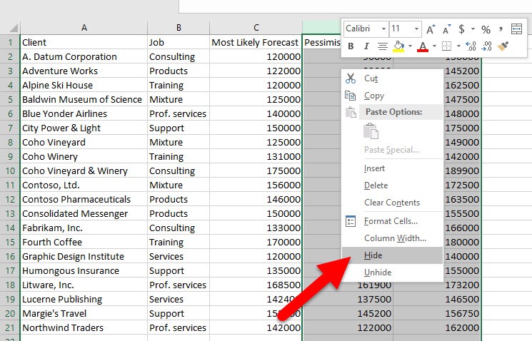
1. Open the worksheet and select the rows or columns of data you want to hide. We’ll select the columns D and E.

2. Right-click the selected rows or columns and from the contextual menu, select Hide.

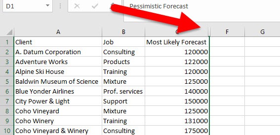
That’s it! The selected rows and columns will disappear from view. You will notice that the column or row headers are missing a few Row numbers or Column Letters and there’s a double-line over the hidden rows or columns.

Should you want to bring back the items you hid previously, you can select the row or column headers adjacent to the hidden ones, right-click the selected columns and from the contextual menu, select Unhide. You can also click and drag the double line over the hidden rows/columns to bring all the hidden rows and columns into view.

How to Hide Data in a Worksheet : Method 2

In the first method of hiding data, all your row and column data will be removed from view. Maybe, that’s not what you want. Maybe you want only some part of the data to be hidden from view. In such a case you can use this method. Let’s hide only the Optimistic revenue figures.

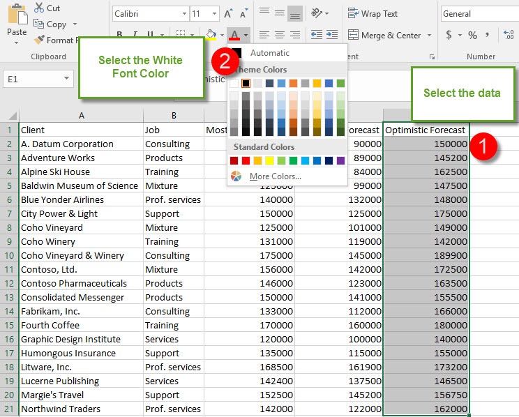
1. Select the range of cells you want to hide. I’ll select the range E1:E21.

2. On the Home tab, in the Font group, click the Font Color drop-down button and select the White color font.

The data you selected is now invisible to the eye. However, you need to remember that the data is still there and if you select a cell with the white font, you will be able to see its contents in the Formula bar.

If you want to display the data again, simply select the cell range ( or the entire worksheet area) and change the font color to black.

One of the dangers of hiding data this way is that should the data be shared with another user, they may easily overwrite the contents by accident. Therefore, make sure you protect your worksheet data by following the steps in this tutorial, which is a safer option.

If you found this tutorial helpful, be sure to check out more good stuff in our Learn Excel series. If you want to learn Excel from scratch, consider taking up our Udemy course, Excel 2016 for Beginners. It is available at a nominal price of just $10.