Learn Excel : How to Remove the First Word from a Cell

In this Learn Excel series, we show you how to remove the first word from a cell containing data. You can use the formulas directly by copying and pasting or you can learn how these formulas work so you can apply it by yourself the next time you’re faced with a similar problem.

How to Remove the First Word from a Cell

To remove the first word from a cell, we make use of the formula:

=RIGHT(A1,LEN(A1)-FIND(” “,A1))

You may also be interested in reading: How to Use Excel Functions in Formulas

In this formula, we assume that the data we want to remove the text from is in cell A1. If that’s not the case, and your data is in another cell, say F2. replace the A1 in the formula with F2.

Again, if you have special characters in your data, say a – between words you want to separate, you need to replace ” “ with the separator the text contains. In this case, you need to add “-“ in your formula instead of ” “. Let’s take a look at an example.

Example to Remove the First Word from a Cell

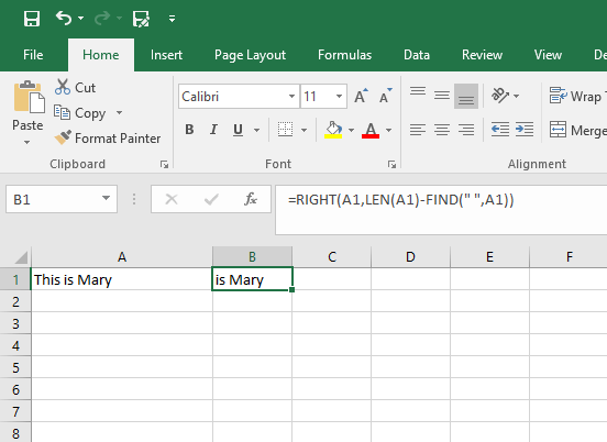
In this example, we have the text “This is Mary” in cell A. In cell B1, we apply the formula, =RIGHT(A1,LEN(A1)-FIND(” “,A1)) to get the result : is Mary.

Now for a bit more explanation on how the function works.

In the formula to remove the first word from the text, there are 3 functions at work: the RIGHT(), LEN(), and FIND() functions.

The RIGHT function works by removing text from the right of the cell. Since we want to extract all of the text except the first word, we make use of this function. But how does Excel know how many characters to remove?

That’s where you use the LEN and the FIND functions.

Now to extract everything except the first word, we need to find the character that separates (separator) the first word from the rest of the text. The FIND function helps to do that.

In this example, the separator is a space. So the FIND function searches for the space to get the number of characters from the left of the cell until the first space.

In our example, this returns 5. That is , 5 characters is what we want to remove from the cell.

Finally, to get the number of characters we want to keep, we use the LEN function. This function counts all of the characters in the cell. The result of the LEN function is 12 because there are 12 characters in the cell, including spaces in between the text.

So, in our formula =RIGHT(A1,LEN(A1)-FIND(” “,A1))  we subtract the result of FIND from that of LEN, which is 12-5=7.

This tells the RIGHT function to get 7 characters from the right of the cell, which removes the first word from the cell.

Now that you know the logic behind how this function works, you can write the formula using this logical function to arrive at a quick solution to your problem.

If you found this tutorial helpful, be sure to follow our Learn Excel series. If you want to learn Excel from scratch, consider taking up our Udemy course, Excel 2016 for Beginners, which is available at a nominal price of just $10.