How to Use Excel Functions in Formulas

In the previous few posts, we discussed how to write Excel formulas, starting with simple ones and moving on to more complex formulas. We also saw how to use absolute and relative referencing in formulas. Today’s topic is all about how to use Excel functions in formulas.

What is an Excel Function?

An Excel function is a small program or predefined formula that can perform specific calculations in a specific order. For example the SUM function totals numbers while the AVERAGE function calculates an average. Excel of course has a large number of functions that can perform calculations for various components such as numbers, text, dates, time and so on. Functions can be performed individually or they can be nested and performed one inside another.

However, functions cannot exist on their own; they always have to be part of a formula. Before you start using functions, it is best to understand the different parts of the function. Excel functions are written a specific format, what we call syntax. The basic syntax of any function starts with an equals sign(=), the function name (COUNT for example), and one or more arguments. Arguments contain further information on what you want to compute. Let’s look at a few example Excel functions.

=SUM(A1:A5) : This is an example of a function acting as a whole formula. It returns the sum of the values in the range A1:A5.

=SUM(A1:A5) /B5 : This is an example of a formula containing a mixture of a function’s result with other data. It returns the sum of the values in the range A1:A5 divided by the value in cell B5.

=SUM(A1:A7) + AVERAGE(B1:B7) : This is an example of a formula that combines the result of two functions. It returns the sum of the range A1:A7 added with the average of the range B1:B7.

Working with arguments

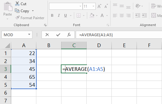
Arguments are always enclosed within parentheses and can refer to data in individual cells or within cell ranges. A formula can contain one argument or multiple arguments, depending on what you wish to calculate. For example, the function =AVERAGE(A1:A5) will calculate the average of the values in the cell range A1:A5. This function contains only one argument.

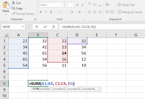
If you write a formula with multiple arguments, the arguments must be separated by a comma. For example, the function =SUM(A1:A5, C1:C4, D1) will add the values of all the cells in the three arguments.

How to Write Excel Functions

Excel has a variety of functions available. We’ll work with some common functions like the ones outlined below:

• SUM: This function adds all of the values of the cells in the argument.
• AVERAGE: This function calculates the average of the values included in the argument.
• COUNT: This function counts the number of cells with numerical data in the argument.
• MAX: This function determines the highest cell value included in the argument.
• MIN: This function determines the lowest cell value included in the argument.

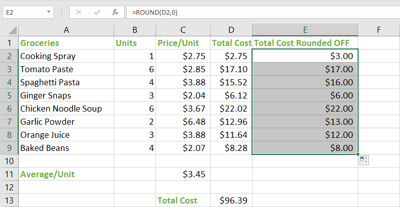
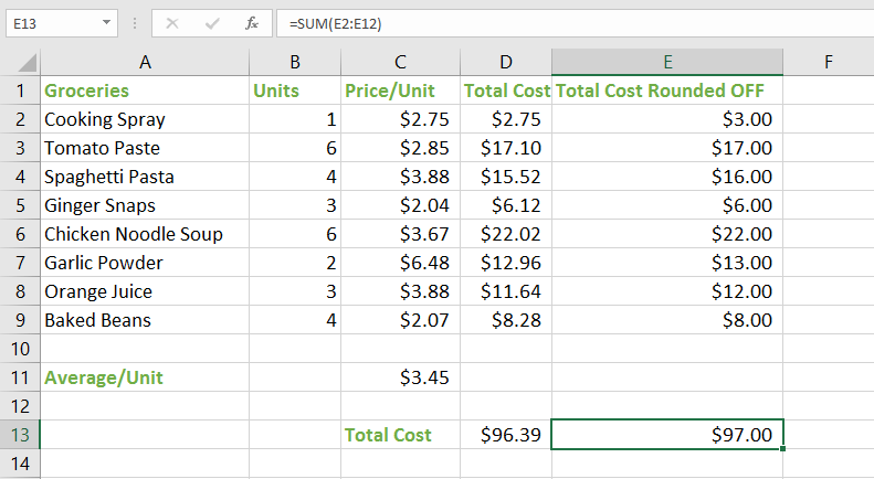
Let us now create a basic function to calculate the average price per unit for the items listed in our worksheet. We will use the AVERAGE function for this.

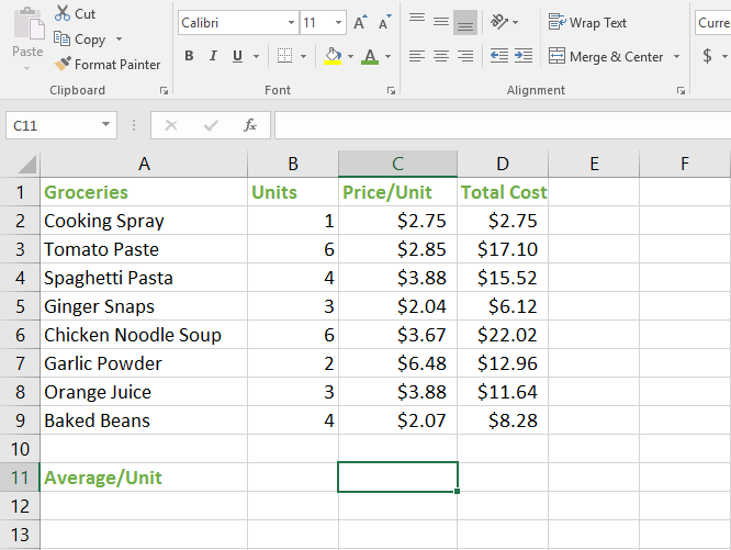
1. Select the cell where you will write your formula. In our example, it is cell C11.

2. Type the equals sign (=) and enter the function name. You can also select the function name from the list of suggestions that appear below the cell as you type. In our example, we’ll type =AVERAGE.

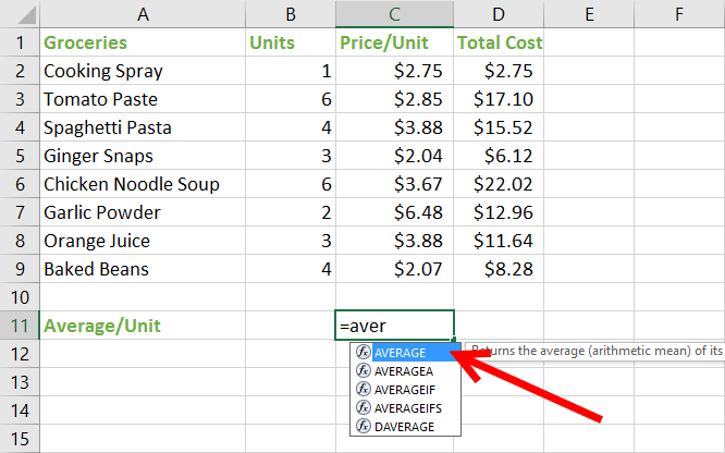
3. Enter the cell range for the argument within parentheses. In our example, we’ll type (C2:C9). This formula will add the values in cells C2 to C9 and divide that sum by the total number of cells in the range to get the average price per unit.

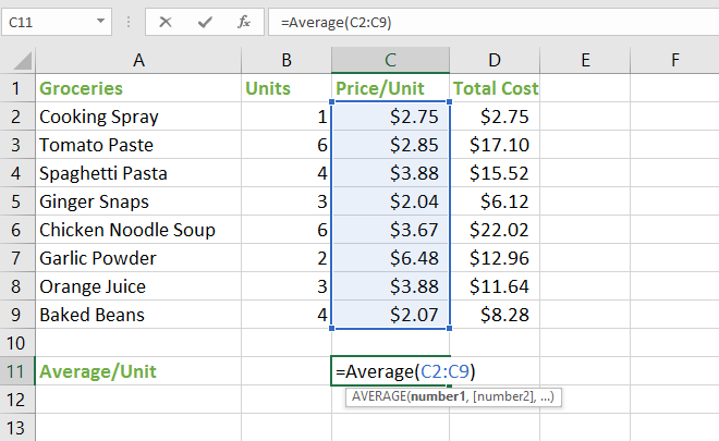
4. Press Enter to get the final value or average price per unit of $3.45.

Let’s now create a function to compute the total cost of the items in the worksheet. For this purpose, we can use the AutoSum command. This command allows you to automatically insert the most common functions into your formula such as SUM, AVERAGE, COUNT, MIN, and MAX.

To create a function using the AutoSum command:

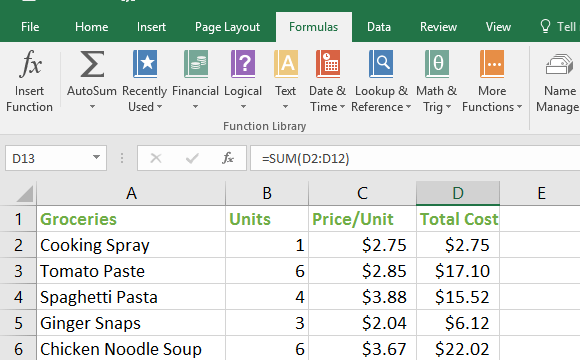
1. Select cell D13 to enter the formula.

2. On the Home tab, in the Editing group, click the AutoSum drop-down and select Sum.

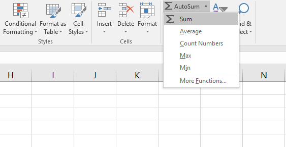
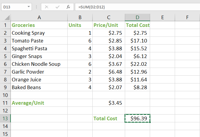
3. The selected function will appear in the cell and will automatically display the cell range selected for the argument. In our example, cells D2:D12 were selected automatically.

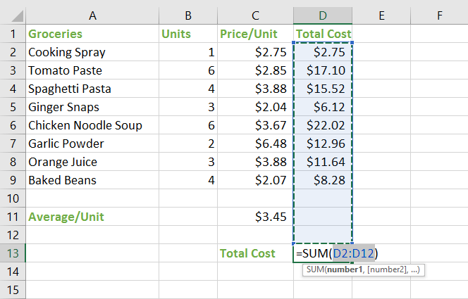
4. Press Enter to let Excel do the math and display the total cost. In my example, it is $96.39.

The Excel Function Library

Excel contains plenty of functions and its impossible to learn all of them. Depending on your work requirements, you can learn about specific functions, but it still doesn’t hurt to be aware of the different types of functions. The Excel Function library, which is available on the Formulas tab displays all the different types of functions by category and you can explore them at your leisure.

How to Insert an Excel Function from the Function Library

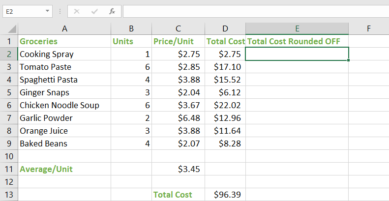
We’ll continue with the current example and round off the individual totals in our worksheet using the ROUND function from the Function Library. To do this:

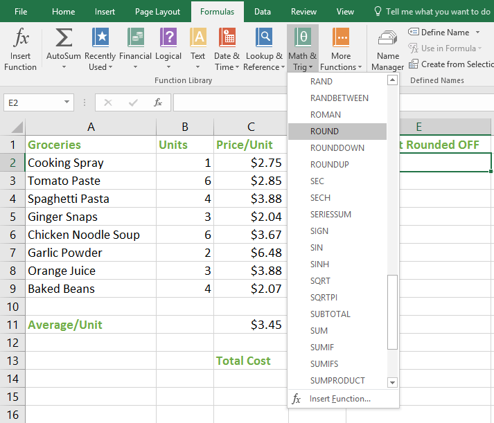
1. Select the cell where you plan to include the formula. In this case it is cell E2.

2. On the Ribbon, select the Formulas tab.

3. In the Function Library group, click the Math & Trig drop-down and select Round.

4. The Function Arguments dialog box is displayed. In the Number text box, you need to enter the number you want to round. Select cell D2. In the Num_Digits text box, select the number of digits you want to round off to. In this case its 0. Click OK to close the dialog.

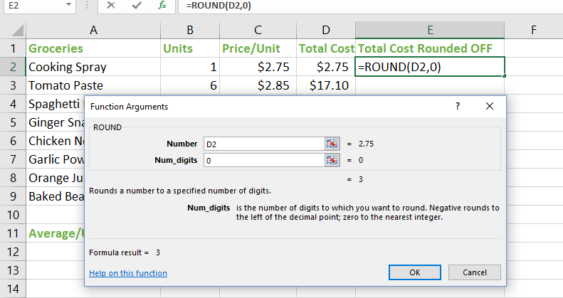
5. The function will be calculated, and the result will appear in cell D2. In our example, it is $3. Use the fill handle to drag down the formula to the remaining cells.

The Insert Function Dialog

If you can’t find the function you need for your formula, you can use the Insert Function dialog box to search for functions using keywords. This dialog will also guide you through the process of entering a function. Here’s a look at how to write a function using the Insert Function dialog:

In this example, we’ll sum up the total cost of items that we rounded off in column E using the commands in the Insert Function dialog.

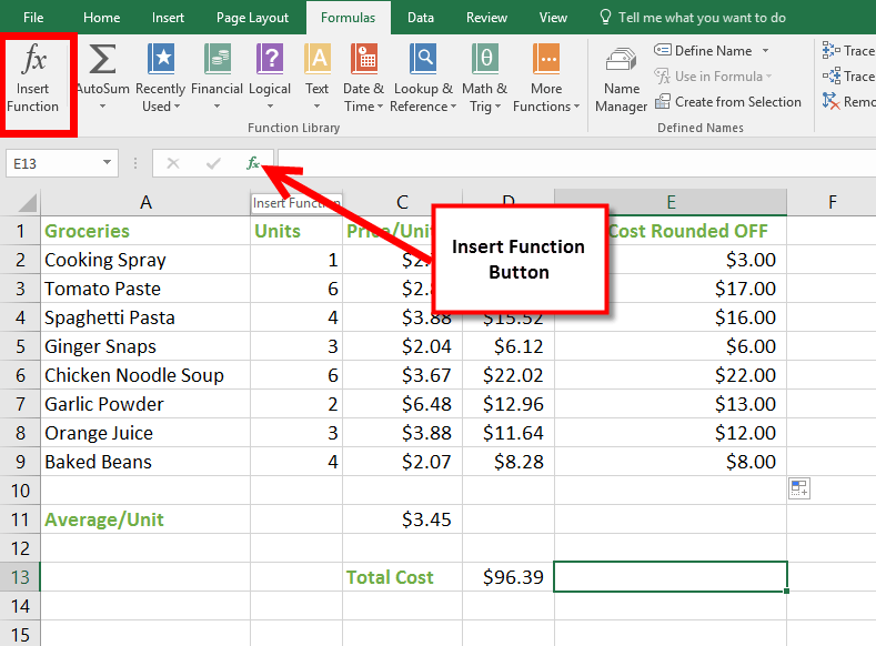
1. Select the cell where you plan to include the formula. In this case it is cell E13.

2. On the Ribbon, click the Formulas tab, click the Insert Function command. Alternately, you can click the Insert Function button on the Formula Bar.

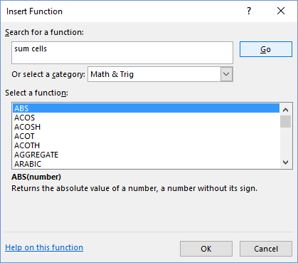
3. The Insert Function dialog box will appear. If you don’t know the name of the function, type a few keywords describing the calculation in the Search for a function text box. If you know what you are looking for and where it is available, you can use the Or select a category drop-down to find it. In our example, we’ll type sum cells in the  Search for a function text box.

4. Review the results to find the function you are looking for, select it and then click OK. In our example, we’ll choose SUM and click OK.

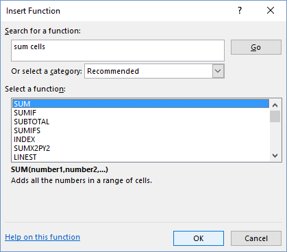
5. The Function Arguments dialog box will be displayed. Select the Number1: field, then enter or select the desired cells. In our example, it is automatically selected. You can continue to add arguments in the Number2: field, but in this case we only want to sum the numbers in the cell range E2:E10. When you’ve added the cell range, click OK.

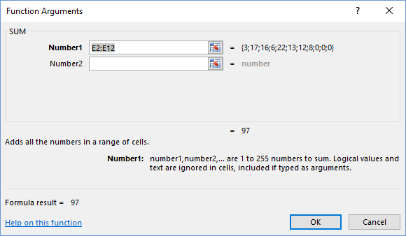
The function will be calculated, and the result will appear in cell E13. In our example, the total cost (rounded OFF) is $97.

You can try working with some more of the basic functions, or try a more advanced one like VLOOKUP. You can check out our article on How to Use Excel’s VLOOKUP Function for more information.