Have you tried entering the ampersand sign in your custom header or footer only to find that it disappears on your printed worksheet? Well, here’s a simple trick on how to enter the ampersand sign in Excel headers and footers that show up on your printed page.
If you are new to creating headers and footers in Excel, you can check out my previous post on how to insert headers and footers in your worksheet. If you have been using headers and footers for some time, but decided to create a custom footer with an ampersand (&) sign and found that your printed copy is missing the sign, here’s what you need to do.
How to Enter the Ampersand Sign in Excel Headers and Footers
Let’s create a A & B Bricks Ltd. as the custom header in our Employee List worksheet.
1. Open the workbook and select the Page Layout tab.
2. In the Page Layout Group, click the dialog box launcher to display the Page Setup dialog box.
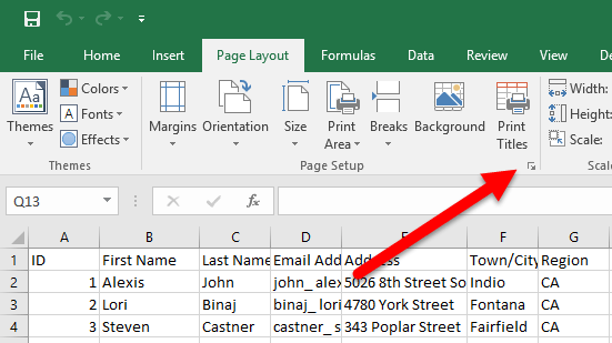
3. In the dialog box, select the Header/Footer tab.
4. Click Custom Header to open up the Header dialog box.
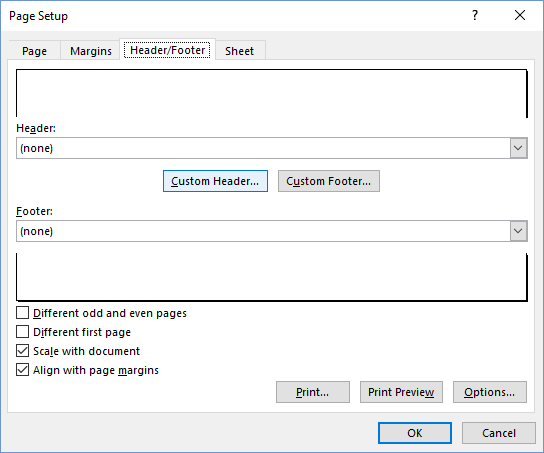
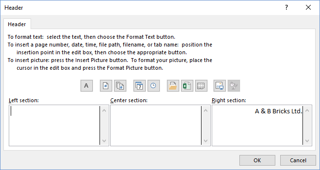
5. Here you have 3 sections to add a custom header. You can enter a header on the left, on the right, or in the center. Let’s enter A & B Bricks Ltd. in the right section and then click OK.
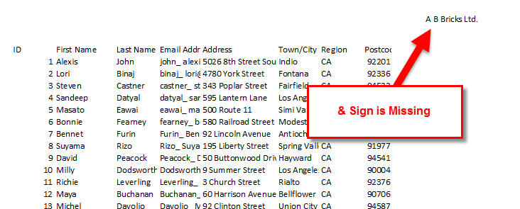
6. Now in the Page Setup dialog box, click Print Preview. Notice that the header information in the print preview is missing an ampersand.
7. Now go back to the Page Setup dialog box and select the Header/Footer tab.
8. Click Custom Header to edit the header information.
9. Now, enter another ampersand sign next to the first one you typed – A && B Bricks Ltd.
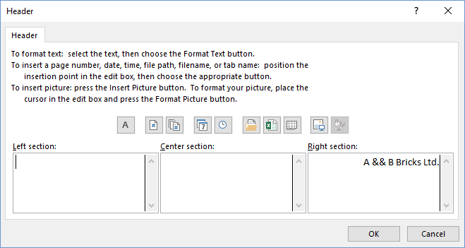
10. Click OK and do another print preview.
The Ampersand sign will now be visible on your preview and print page.
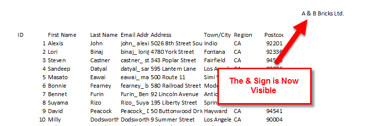
You can follow the same procedure to add ampersand sign to your footer also. That’s it! A simple trick to get the & sign to show up on your printed worksheets!
If you’d like to know more Excel tips and tricks, please visit our Archives section and if you want to learn all the basics of Excel, check out our Udemy course as well!
Leave a Reply