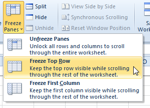
Working with large worksheets becomes tiresome if you have to keep scrolling up and down the worksheet multiple times to look for specific data. The Freeze Panes command in Excel 2010 allows you to freeze certain rows and columns so that they remain static while you scroll through the rest of the spreadsheet. This is mainly used when you have row and column headers that you want to view while scrolling through the length and breadth of the worksheet. In this Excel 2010 tutorial, you will learn how to freeze rows and columns in a worksheet.
Restrictions of Freezing Rows and Columns
There are certain limitations in freezing rows and columns.
1. You can freeze rows only from Row 1 and columns from Column A. For example, if you freeze row 50, rows 1-49 will also be in the freeze state.
2. You cannot freeze rows or columns in the middle of your worksheet without freezing the rows or columns that are above and to the right of the selected cell.
3. If your worksheet is protected then you cannot freeze the panes.
4. You cannot freeze a worksheet when it is in the cell editing mode.
How to Freeze Rows and Columns in a Worksheet
How to Freeze the Top Row of a Worksheet
1. On the View tab, in the Window group, click Freeze Panes.
2. In the drop-down list, select Freeze Top Row.
How to Freeze the First Column of a Worksheet
1. On the View tab, in the Window group, click Freeze Panes.
2. In the drop-down list, select Freeze First Column.
Note: You cannot freeze both the top row and the first column using the above commands. You can either freeze the first row or freeze the first column. For example, if you froze the first row and then proceeded to freeze the first column, the freeze action on the first row will get undone.
How to Freeze Both Rows and Columns in a Worksheet
1. Select a cell below and to the right of the cells you want to freeze. For example, if you want freeze from row 5, and from column 2, select cell C6.
2. On the View tab, in the Window group, click Freeze Panes.
3. In the drop-down list, select Freeze Panes.
Note: You can also use the Freeze Panes command to freeze multiple rows or to freeze multiple columns. However, you need to remember that you can only freeze cells right from row 1 or column A.
How to Unfreeze a Row or Column in a Worksheet
1. On the View tab, in the Window group, click Freeze Panes.
2. In the drop-down list, select Unfreeze Panes.
In this Excel 2010 tutorial, you learned how to freeze rows and columns. This will enable you to view specific rows and columns when scrolling through large worksheets.

Leave a Reply