When you want to derive specific information out of a big Excel database, the Excel VLOOKUP function is one of the most handy features that you can take advantage of. For a first time user of the function, VLOOKUP may sound intimidating.
That’s because you most often end up with all sorts of errors that can baffle you. But once you understand the workings of this popular Excel function, you will be able to confidently look up any data on a spreadsheet of any size. This Excel VLOOKUP tutorial features a couple of examples that will help users understand and try out the steps themselves.
Introduction to Excel VLOOKUP
VLOOKUP is an Excel function that searches your workbook for a value that you specify to return a matching value from another column in your workbook. In other words, it looks through your lists or table data for a unique item (that you are searching for) and pulls up a piece of information that is associated with that item. VLOOKUP stands for vertical lookup meaning that it can look up values in vertical columns.
Excel VLOOKUP Explained with an Example
VLOOKUP is best explained and understood using examples. Here is a basic scenario where Excel VLOOKUP can be applied.
You have an Excel Sheet (Employees Payroll.xlsx) with a list of employees in your firm with their hourly wage rates. Your personal assistant has just sent you another worksheet (Employee Work Hours.xlsx) showing the number of hours put in by each worker at the end of the week. However, the list of workers are not in the same order in which you have them in your Employees Payroll worksheet.
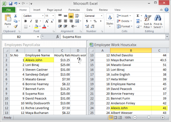
In this scenario, you can use VLOOKUP on your worksheet to pull out the hours worked by each employee from the Employees Payroll worksheet.
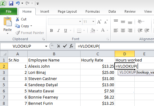
Once you lookup the value of one employee, you can simply use the filler to drag down the rest of the values.
The VLOOKUP Function – Its Syntax and Rules
The VLOOKUP function carries the following syntax:
VLOOKUP( lookup_value, table_array, col_index_num, [range_lookup] )
This might look quite confusing to a new user of the function, but here’s what each of its arguments means.
- lookup_value : This is the value that you are using to search for information related to it.
- table_array: This is the table of data where you need to search to find the corresponding lookup value. The VLOOKUP function normally searches for this in the left-most column of the table_array.
- col_index_num: This is the column number of the table_array from where you want to return a value from.
- [range_lookup]: This is an optional logical argument that can be set to TRUE or FALSE. TRUE indicates to find the closest match below or equal to the lookup value if the exact value is not found. If you don’t enter a range_lookup value, this is usually set to TRUE. FALSE indicates to find the exact match to the lookup value and if not found return an #N/A error.
You can find a handy reference card explaining the VLOOKUP syntax at the Microsoft website.
Example 1: Using VLOOKUP Function in an EXACT MATCH scenario
In the example above, we had two Excel sheets, Employees Payroll.xlsx and Employee Work Hours.xlsx. The Employees Payroll worksheet contains names of employees and their wages. The Employee Work Hours contains the exact same employees in a different order with their hours of work.
Your task is to compute the wages of each employee. For this purpose, you need to open up Employees Payroll worksheet, create a VLOOKUP function to look up the hours worked by the employees, which is available in Employee Work Hours. Then compute the wages in the Employees Payroll worksheet. Let’s do the VLOOKUP now.
You can download the sample files used in this VLOOKUP tutorial below.
Download Employees Payroll.xlsx and Employee Work Hours.xlsx
1. Open both Employees Payroll.xlsx and Employee Work Hours.xlsx worksheets.
2. In Employees Payroll.xlsx, click inside cell D2.
3. Type = and in the Formula bar, click the drop-down arrow and select More Functions.
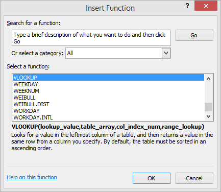
4. In the Insert Function dialog box, scroll down and select VLOOKUP and click OK.
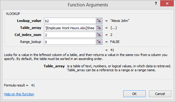
5. In the Function Arguments dialog box, in the Lookup_value field, enter B2. This is the name of the employee you want to lookup.
6. Click inside the Table-array text box. Now navigate to Employee Work Hours.xlsx worksheet and click on columns B and C. You are in effect creating a table array with the employee name as the first column and the hours worked as the second column.
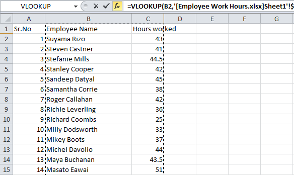
7. Click inside the Col_index_num text box, and enter 2. This is because in your table array, you are looking for the values in column 2 (the hours worked).
8. In the Range_lookup dialog, enter 0. This value equals FALSE, meaning that if VLOOKUP is not able to find an exact match, it should return the #N/A error.
This is what your Function Arguments dialog box should look like now.
9. Click OK.
Now on your Employees Payroll.xlsx, you will be able to see the hours Alexis John worked, i.e 41 hours displayed against his name. Click in cell D2 and drag down the fill handle to match the rest of the employee names against their work hours.
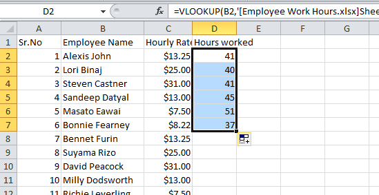
That’s it. You have just learned how to create your first VLOOKUP table. That wasn’t too hard was it?
Example 2: Excel VLOOKUP Tutorial in CLOSEST MATCH Scenario
Let’s take a look at another example, this time to match the Range_lookup argument to TRUE. Remember that when you set the [range_lookup] argument to TRUE, it will return the closest match below that of the lookup value when it cannot find an exact match.
Also, in this type of scenario, the left-hand column of the table_array must be in ascending order for the VLOOKUP function to work correctly.
In this example, we have a worksheet called Quantity Discounts.xlsx containing a table of discounts for quantities sold. Also in the sheet are a couple of fields, Quantity and Discount that should help you compute the discount for a specific quantity of items sold. Your task is to create a VLOOKUP function in cell E3, corresponding to Discount so that you can instantly find the discount applicable for any quantities you may input in cell B7.
In this scenario, you are not looking for an exact match, but the closest match. That’s because quantities sold will vary from customer to customer and your discount rates apply for a range of goods.
You can download the sample files used in this VLOOKUP tutorial below.
Download Quantity Discounts.xlsx
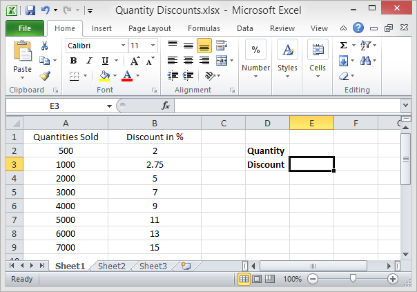
1. In the Quantity Discounts worksheet, click inside cell E3.
2. Type = and in the Formula bar, select VLOOKUP.
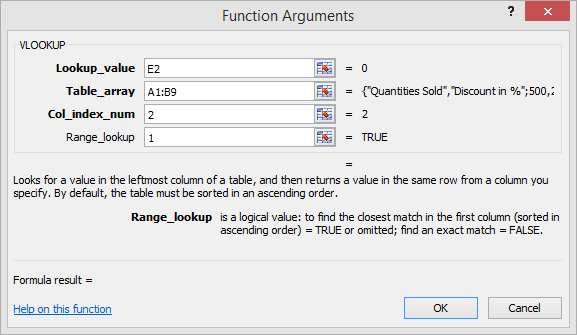
3. In the Function Arguments dialog box, in the Lookup_value field, enter E2. This is the quantity of goods sold.
4. In the Table-array text box, enter the range A1: B9. Or you can drag your mouse over cells A1 to B9 in the worksheet.
5. In the Col_index_num text box, and enter 2. This is because in your table array, you are looking for the values in column 2 (the discount percentage applicable).
6. In the Range_lookup dialog, enter 1. This value equals TRUE, meaning that if VLOOKUP is not able to find an exact match, it should return the value below that of the lookup value.
This is what your Function Arguments dialog box should look like now.
9. Click OK.
Now your worksheet will contain the VLOOKUP function displaying an #N.A error. That’s because you are yet to input the quantity value in column E2.
Now lets say you sold 2550 units and need to find out the discount applicable on it. Just input 2550 in cell E2 and VLOOKUP will automatically show up the discount %.
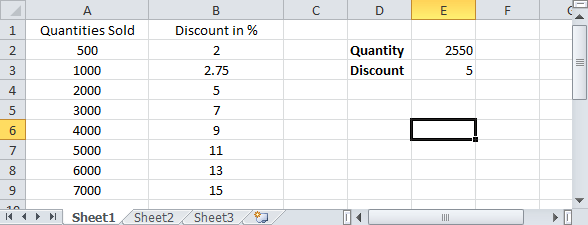
So we have seen two scenarios where VLOOKUP can be used successfully. Now that you have gained a basic understanding of how VLOOKUP works, you can go ahead and start using them in your day to day work.
Common VLOOKUP Errors
The VLOOKUP function can get frustrating to use on account of the sheer number of times you end up with errors. And all the help topics in the world may not make sense to you at that point. So lets take a look at some of the common reasons you end up with VLOOKUP errors.
Encountering and Fixing an #N/A error
#N/A errors can occur in a number of different situations. Here are some common instances and solutions to fix them.
Situation : Lookup value not found
Solution: A possible cause for this could be typos or spelling errors in your lookup values
Situation : #N/A error shows up when you set the range_lookup argument to TRUE
Solution: This could be due to the fact that the lookup value is smaller than the lowest value in the table array or due to the fact that the lookup column is not in ascending order.
Situation : #N/A error shows up when you set the range_lookup argument to FALSE
Solution: This could be due to the fact that there is no exact value to match.
Situation : Lookup Column is not to the left
Solution: VLOOKUP cannot read values to its left. Therefore if you do not set your lookup column to the extreme left in the table array, you will end up with this type of error.
Improper Formatting of Data
For example, if you imported data from another source like a website, you may end up with numbers being formatted as text, causing the errors. Simply format the data as numbers to eliminate the problem.
Leading or Trailing Spaces in Table
Removing these extra spaces using the TRIM function will automatically eliminate these errors.
Encountering and Fixing #VALUE errors and #REF errors
Another frequent error that you are likely to encounter is the #VALUE error. This happens when a value that is used in the function is of a wrong data type. There are times when a simple space can cause such errors, in those scenarios you can follow the remove spaces in excel tutorial to get a quick fix.
Situation: Lookup value is more than 255 characters
Solution: Although an unlikely scenario, VLOOKUP cannot look up values beyond 255 characters.You may have to use another formula instead.
Workbook Path Incorrect
If you are pulling data from another workbook, you must indicate the full path to that workbook. For instance, you must place the name of the workbook along with its extension in square brackets and then mention the sheet’s name followed by the exclamation mark. Also, you should have apostrophes if the names contains spaces.
col_index_num argument is less than 1
Although this is a rare occurrence, you might want to avoid specifying the column to return values to less than 1.
VLOOKUP displaying a #REF error
This typically happens when your col_index_num argument is greater than the number of the columns in the specified table array.
I hope this Excel VLOOKUP tutorial helped you gain a better understanding of what VLOOKUP is, how it can be used in various situations and how you can avoid the common errors in VLOOKUP.
Leave a Reply