One of the common tasks we perform when working with large Excel worksheets is filtering data in alternate rows. This may be for the purpose of further analysis, or we may just want to delete such data. Whatever the reason, there’s no simple auto filter option that lets you filter alternate rows in Excel directly. The cool thing with Excel is that most tasks are still doable. So here’s one way to filter alternate rows in Excel 2010.
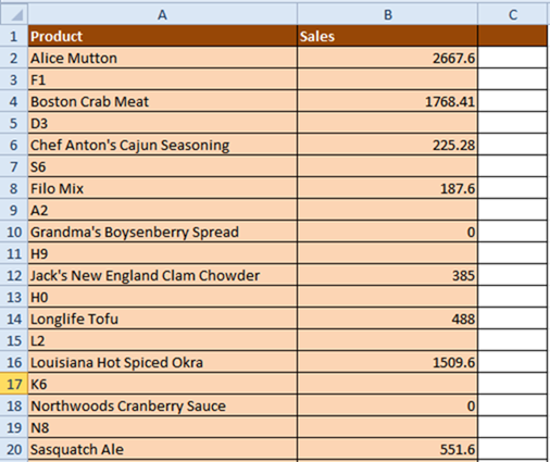
In the graphic below, we don’t want the data that is displayed in rows 3, 5, 7, 9, 11, 13, 15, 17 and 19. We need to filter the alternate cells containing the unwanted data and delete them. To do this simply follow these quick steps.
How to Filter Alternate Rows in Excel
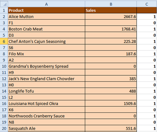
1. In another column, or in this scenario, in Column C, in cell C2, enter the formula =MOD(ROW(A1),2)
If you want to change every 3rd row, change the 2 in the formula to 3. Similarly, if you want to filter every 5th row, change 2 to 5.
2. Using the Auto fill functionality, drag the bottom left corner of the cell to cell C20. The column will display the values 1 and 0 in alternate succession. This will change to 1, 2, and 0 when you want to filter every 3rd row, and 1, 2, 3, 4, 0 when you want to filter every 5th row.
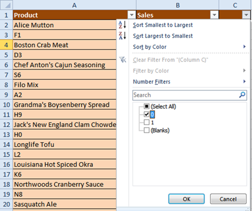
3. Click the title row. In this case, select Row 1. Then select the Data tab. In the Sort & Filter group, click Filter. The filter button is added to all the titles.
4. In column C1, click the filter arrow and select 0 and click OK.
Volia! You’ve just filtered the alternate rows in Excel. Now just select the cells and hit the Ctrl+Minus button to delete the alternate rows.
A quick and easy way to get rid of unwanted data sitting in nth row of a worksheet. I find this happening when I copy data from a web page to Excel and now removing the unwanted rows is a breeze.
Follow us on Twitter, Facebook or Google +to get the latest tutorials, updates and how-to articles on Microsoft, Google and Apple products.


Leave a Reply