Excel offers a number of handy tools to sum up the totals of all the numbers in a range of cells in your worksheet. But what about those times when you only want to sum up specific values in a range? In such situations, you can make use of the SUMIF and SUMIFS functions. In this Excel tutorial, I’ll show you how to use these math functions to add together just the values you want to sum.
How to Sum Up Specific Values in a Range Using SUMIF
The SUMIF function lets you command Excel to sum up the numbers in a particular range of cells only if it meets a specific criteria you specify. The SUMIF syntax looks like this:
=SUMIF (range, criteria, [sum_range])
where:
range = the range of cells you want Excel to consider when summing.
criteria = condition for evaluating whether to include certain values in the range when summing
sum_range = this is an optional value and includes the actual cells to be summed. If you don’t include this optional argument, Excel only sums the first range you specified, provided they meet your criteria.
Let’s understand this with the help of a simple example.
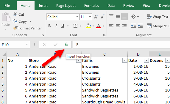
In our Daily Sales worksheet, we have a list of stores with various goodies sold at each of these locations at various dates. We also have the daily sales generated at each of these locations. Let’s say we wanted to find the total sales of Brownies in all the locations and input the total sales in cell J2. We can use the SUMIF function as follows:
1. Place the cursor in cell J2. Then click the Insert Function dialog box on the Formula Bar.

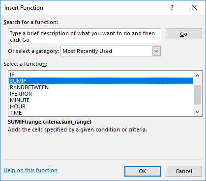
2. In the Insert Function dialog box, in the Search box, type SUMIF and press Enter. In the Select a function box, check if SUMIF is selected.

3. Click OK to display the Function Arguments dialog box.
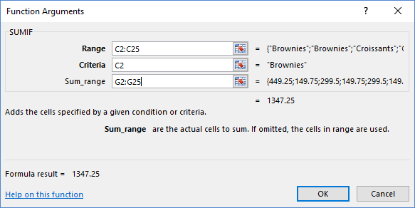
4. In the Function Arguments dialog box, you can see the arguments I spoke about in the syntax earlier. Enter the values as specified.

Range: the cells you want to consider, which is the range C2: C25.
Criteria: is the condition for evaluating whether to include certain values. This is Brownies, which is C2.
Sum_range= this is an optional value and includes the actual cells to be summed. In this case, it is the daily sales, which is the range G2:G25.
5. Once you’ve entered the values click OK.
You will instantly see the daily sale of Brownies across all locations.
If you wanted to find the total sales of another item say Sandwich Baguettes, you’d substitute C2 with C6 or simply type Sandwich Baguettes in the Criteria text box to get the result.
How to Sum Up Specific Values in a Range Using SUMIFS
The SUMIFS function works exactly the same as the SUMIF function, except that it lets you add more than one criteria range. Its syntax looks slightly different:
=SUMIFS (sum_range, criteria_range, criteria, …)
where:
sum_range = the actual cell range you want to sum
criteria_range = cells with all entries that need to considered by the if criteria
criteria = the condition applied to the criteria_range to decide which values to total.
Let’s understand how this works using an example. We’ll use the same worksheet Daily Sales. This time, we’ll calculate the sale of Brownies in just one location, say Cedar Street and enter the value in cell J8. To do this:
1. Place the cursor in cell J8. Then click the Insert Function dialog box on the Formula Bar.
2. In the Insert Function dialog box, in the Search box, type SUMIFS and press Enter. In the Select a function box, check if SUMIFS is selected.
3. Click OK to display the Function Arguments dialog box.
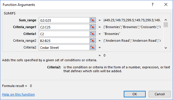
4. In the Function Arguments dialog box, enter the values as specified.

Sum_range: the actual cell range you want to sum, which is the daily sales, G2: G25.
Criteria_range1: is the condition to be used in evaluating whether to include certain values. We want to include the range of items here, which is C2:C25.
Criteria1 : This is the condition that defines the criteria of cells to be summed. In this case, it is Brownies, which is C2.
Criteria_range2: is the condition for evaluating whether to include certain values. We want to include the location range, which is B2:B25.
Criteria2: This is the condition that defines the criteria of cells to be summed. In this case, it is the location, Cedar Street, which is B18. You can alternately just type the street name.
5. Once you’ve entered the values click OK.
You will instantly see the daily sale of Brownies in Cedar Street.
Using the SUMIF and SUMIFs functions is quite easy and helps you quickly sum up specific values in a range of cells in your worksheet. If you are comfortable with using the function syntax, you can enter the arguments directly, but if you’re a newbie, using the Insert Function box helps you accomplish the task more easily.
If you wish to practice the functions, click below to download the worksheet and try using the function on different items and locations.
Leave a Reply