Yesterday, I explained how you can use a combination of Excel functions to remove the first word from a cell. Today, in our Learn Excel series, we take a look at how to remove the last word from a cell. Again, you can simply copy and paste the formula to get the result or you can read on to understand how the formula works so you can apply it using your logic in any given situation.
How to Remove the Last Word from a Cell
To remove the last word from a cell, we make use of the formula:
=LEFT(A1,FIND(“~”,SUBSTITUTE(A1,” “,”~”,LEN(A1)-LEN(SUBSTITUTE(A1,” “,””))))-1)
You may also be interested in reading: How to Use Excel Functions in Formulas
In this formula, the data we want to remove the text from is in cell A1. If that’s not the case in your worksheet, say you data is in cell G2, replace the A1 in the formula with G2.
Also, if you have special characters in your data, say a – between words you want to separate, you need to replace ” “ with the appropriate separator. In this case, you need to add “-“ in your formula instead of ” “. Let’s take a look at an example.
Finally, if you data uses the ~ (tilde), then replace the ~ in the formula with another character that is not in your data.
Example to Remove the Last Word from a Cell

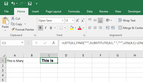
In this example, we have the text “This is Mary” in cell A1. In cell C1, we apply the formula, =LEFT(A1,FIND(“~”,SUBSTITUTE(A1,” “,”~”,LEN(A1)-LEN(SUBSTITUTE(A1,” “,””))))-1) to get the result : This is.
Now here’s the explanation on how the function works.
In the formula to remove the last word from the text, there are 4 functions at work: LEFT(), LEN(), FIND(), SUBSTITUTE().
This can be slightly tedious so bear with me.
The LEFT function works by getting all of the words that are to the left of the last word. Therefore, we need to tell the LEFT function how many characters from the left of the cell we want to extract. But how does Excel know how many characters to remove?
This is where the formula gets tricky. Let’s look at smaller chunks of the formula that helps us find the characters. The formula is FIND(“~”,SUBSTITUTE(A1,” “,”~”,LEN(A1)-LEN(SUBSTITUTE(A1,” “,””))))-1)
Here, (SUBSTITUTE(A1,” “,””)))) does the job of removing all the spaces in the cell. Then it counts the number of characters that are in the left using the LEN function. Hence, LEN(SUBSTITUTE(A1,” “,””)).
In our example above, this result is 10. (thisismary=10)
Then, it counts how many characters are in the cell when the spaces are left in it; that’s the next bit of the formula: LEN(A1). This time the result is 12.(this is mary=12).
Next, the formula subtracts the two results (12-10) to get 2. LEN(A1)-LEN(SUBSTITUTE(A1,” “,””)).
This result is the total number of spaces in the cell. This tells the first SUBSTITUTE function which space to replace. Replace the last space since its a lot easy to find it.
So using the number we just got, we use the SUBSTITUTE function again to replace the last space in the cell with ~ . [SUBSTITUTE(A1,” “,”~”,LEN(A1)-LEN(SUBSTITUTE(A1,” “,””))))-1) ]
Finally, we use the FIND function to find the ~ we substituted. [FIND(“~”,SUBSTITUTE(A1,” “,”~”,LEN(A1)-LEN(SUBSTITUTE(A1,” “,””)))) ]
Now the formula knows how many characters from the left of the cell the last space is.
The formula then subtracts 1 from that number since you don’t want to include the last space in the result. FIND(“~”,SUBSTITUTE(A1,” “,”~”,LEN(A1)-LEN(SUBSTITUTE(A1,” “,””))))-1
Now, we have the total number of characters from the left of the cell right up to the space that comes before the last word. Now the LEFT function will return everything except the last word.
=LEFT(A1,FIND(“~”,SUBSTITUTE(A1,” “,”~”,LEN(A1)-LEN(SUBSTITUTE(A1,” “,””))))-1)
If you find this all confusing, just copy the formula and adjust the cell references in your data. Its a lot quicker and easier.
If you found this tutorial helpful, be sure to follow all the tutorials in our Learn Excel series. If you want to learn Excel from scratch, consider taking up our Udemy course, Excel 2016 for Beginners, which is available at a nominal price of just $10.
Leave a Reply