Understanding Relative and Absolute Cell References in Excel

As we learned in our post on Excel for Beginners, Excel formulas can be constructed using cell references. You can reference cells or a range of cells in a worksheet, other worksheets, or even other workbooks. There are 2 main types of cell references in Excel; Relative and Absolute cell references and both behave differently when copied to other cells. Relative references change when a formula is copied to another cell while Absolute references remain constant when they are copied. Let’s learn a little bit more about what Relative and Absolute Cell References are in Excel.

Understanding Relative and Absolute Cell References

What are Relative References?

By default, cell references in Excel are relative references. That’s because when you copy a formula across multiple cells, they change based on the relative position of the rows and columns. For example, if you copy the formula B1+D1 from row 1 to row 5, the formula will reference the relative location of the row and column to become B5+D5. Relative references are ideal to use when you want to repeat the same calculation across multiple rows or columns.

How to Write a formula Using Relative References

Let us create a formula to compute the total sales value of the products listed in Column A. For this purpose we need to multiple the values in Column B with the values in Column C and get the totals in Column D. Instead of writing the formula for each row individually, we can write the formula just for the first item and then use relative references to do the calculations for the rest.

To start constructing the formula:

1. Click inside cell D2 to enter the formula.

2. Type =

3.  Click inside cell B2, enter the multiplication symbol and then click cell C2 to enter the formula =B2*C2.

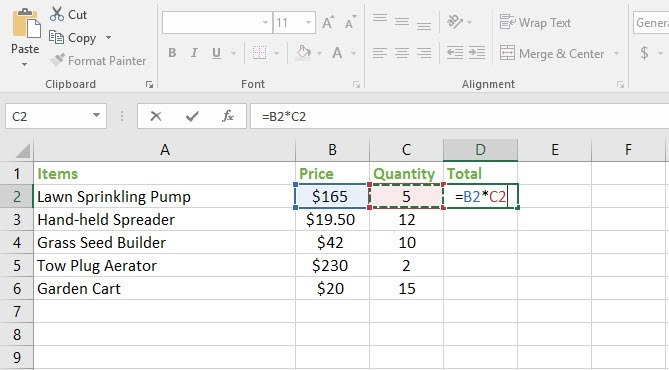
4. Press Enter to get Excel to display the calculated result in cell D2, which is $825.

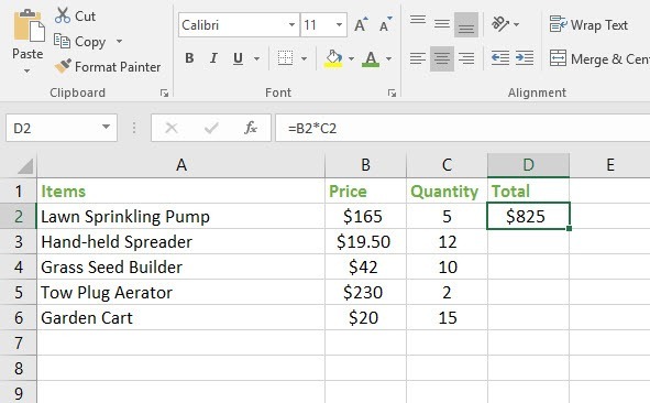
5. Click in cell D2 and drag the fill handle (at the bottom left of the cell) to cell D6.

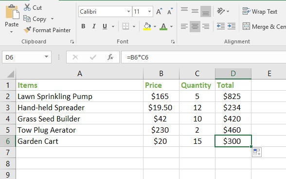
The formula is now copied to cells D3, D4, D5 and D6 using relative references. If you click inside cell D3 and take a look at the Formula Bar, you will see that the formula references =B3*C3; if you click inside cell D4, the formula references =B4*C4; if you click inside cell D5, the formula references =B5*C5; and so on.

What are Absolute References?

There may be times when you do not want Excel to adjust one or more parts of the cell reference in the copied formula. That’s when you use absolute references. Unlike relative references, absolute references do not change a row or column when copied to another cell. A formula containing an absolute reference will have a dollar sign ($) appended to it depending on which part of the reference is absolute or fixed.

Here’s how absolute references will look like.

When you are writing a formula, you can press the F4 key on your keyboard to quickly insert an absolute reference and easily switch between relative and absolute cell references.

How to Write a Formula Using Absolute References

Let’s use the same example we used previously. Now we’ll compute the value of sales tax of each item and input it in column E. For this purpose, we’ll assume a tax rate of 7.5% and include this percentage in column E1. Since all items in the table is using the same tax rate, we want cell E1 to remain absolute in the formula when it is copied to other cells. Therefore we will use the absolute cell reference $E$1 in our formula.

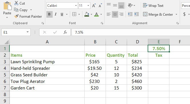
To compute the sales tax:

1. Click inside cell E3 where you want to enter the formula.

2. Type=

3. Click cell D3, enter the multiplication sign, then click inside cell E1 and finally press the F4 key on your keyboard.

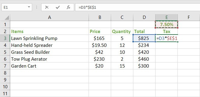
4. Press Enter to get the sales tax value in cell E3.

5. Click inside cell E3 and drag the fill handle right down to cell E7 to get Excel to compute the sales tax value for the rest of the items in the table.

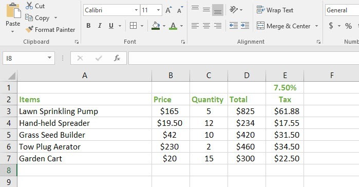
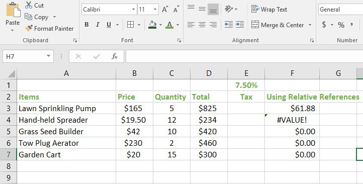
If you were to use relative references to compute the sales tax, as seen in the figure below in column F, you would have ended up with incorrect values.

Using Cell References in Multiple Worksheets

You can use cell references within a worksheet as well as multiple worksheets. In such a case you simply need to reference the worksheet name and add an exclamation point (!) to the formula. Let’s say you wanted to reference cell A1 in Sheet2, your cell reference will be Sheet2!A1.

If your worksheet name has a space, say Sheet 2, you must add a single quotation mark (‘ ‘) around the name. So the cell reference in this case will be ‘Sheet 2’!A1.

How to Reference Cells across Worksheets

In our example below, we’ll refer to a cell with a calculated value between two worksheets. This will allow us to use the exact same value on two different worksheets without rewriting the formula or copying data between worksheets.

In this example we have 2 worksheets. Worksheet 1 is titled Garden tools and contains information about the sales made in the Garden department. Worksheet 2 is called Total Dept Sales and contains sales values of all the departments in the company. Worksheet 2 is however, missing the sales value from the Garden department.

 

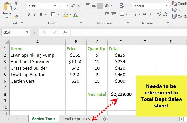
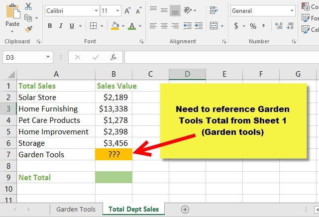
Let’s reference it now.

1. Navigate to the Total Dept Sales worksheet.

2. Click inside the cell where you want to reference the total sales value of the garden tools. In this case, it is cell B7.

3. Type =, enter the sheet name within single quotes and followed by an exclamation point (!) and the cell address. In this example it is =’Garden Tools’!D8.

Alternatively, you can type=, select Sheet Garden Tools, and click cell D8 and press Enter.

The value of the referenced cell will now appear in cell B7. If the value of the sales in Garden tools worksheet changes at any time, it will automatically be updated in the Total Dept Sales worksheet.

Hopefully, this post was helpful in understanding relative and absolute cell references and can apply them confidently in your work.