How to Calculate the Number of Work Days Between Two Dates in Excel

If you use Excel to calculate payment schedules in Excel, one of the most important calculations you do will involve computation of dats between dates. For this purpose you may want to exclude weekends, holidays and other specific days. Thankfully there’s a really useful function in Excel that lets you do the math in a few quick steps. In this Excel tutorial, let’s learn how to calculate the number of work days between two dates in Excel.

Function to Calculate the Number of Work Days Between Two Dates

In order to calculate the number of work days between two dates in Excel, we use the NETWORKDAYS() function. Here’s the syntax for the function:

=NETWORKDAYS(start_date, end_date, [holidays])

Here’s an explanation for this syntax.

Start_date : This is the starting date of the calculation.  This must be entered in the date format but you can also reference a cell that contains a date instead.

End_date: This is the ending date of the calculation.  This must be entered in the date format but just like the start date you can also reference a cell that contains a date instead.

[Holidays]: If you have a list of holidays that you want to exclude from the calculation, enter the range here. Note that the squared brackets indicate that this argument is optional. If you don’t have any dates to exclude, you can leave this argument off the function.

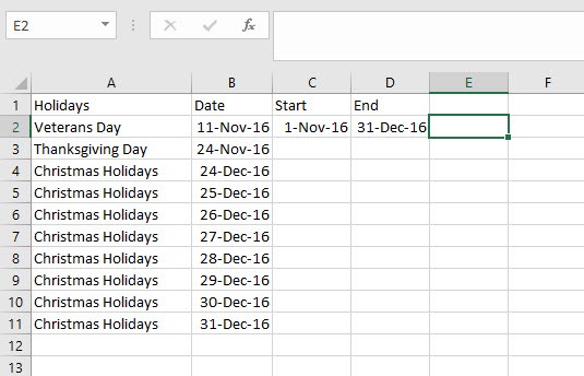
Here’s an example to show how to calculate the number of work days between two dates in Excel. In the sample worksheet, let’s find the number of working dates from 1st Nov 2016 to the end of the year. Column A and B contains a list of holidays that I want to exclude from my calculation. Cells C2 and D2 have the start and end dates respectively.

How to Calculate the Number of Work Days Between Two Dates in Excel

Now to compute the number of work days and enter the result in cell E2, here’s what I need to do:

1. Click inside cell E2.

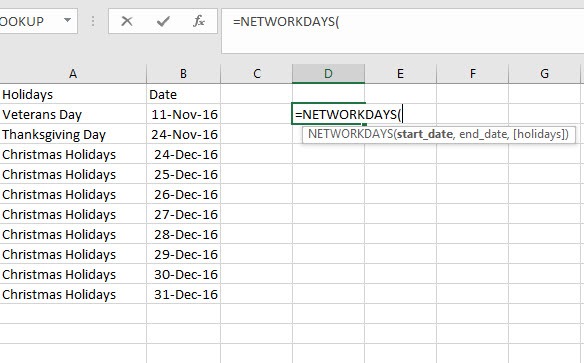
2. Type=NETWORKDAYS(

You can also select the formula that is displayed in the Autosuggestion list.

3. Enter the start date for the calculation, which is in cell C2. The function will now read : =NETWORKDAYS( C2

4. Type a comma. The function will now read : =NETWORKDAYS( C2,

5. Enter the end date for the calculation, which is in cell D2. The function will now read : =NETWORKDAYS( C2,D2

6. Type a comma after the end date.The function will now read : =NETWORKDAYS( C2,D2,

7. Finally, select the range of holidays, that is cells B2:B11. The function will now read : =NETWORKDAYS( C2,D2, B2:B11

8. Close the bracket and hit Enter.The function will now read : =NETWORKDAYS( C2,D2, B2:B11)

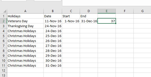
This will give you the result of 37 days. Note that this will also exclude all weekdays within the given date range.

So the next time you want to calculate the number of work days between two dates in Excel, just use the simple NETWORKDAYS function to get the job done. Just make sure you keep your holiday dates refreshed and updated every year so that you don’t have issues with the work day computation.

If you found this tutorial helpful, be sure to read all our tutorials in the Learn Excel series. If you want to learn Excel from scratch, consider taking up our Udemy course, Excel 2016 for Beginners, which is available at a nominal price of just $10.