Excel 2010: How to Summarize Data by Creating PivotTables

If you have a long list of raw data that you want to summarize, PivotTable is the tool for you. Pivot Tables help you to dynamically analyze the relationships between different types of data stored in Excel. The introduction of Slicers in Excel 2010 has made the use of Pivot Tables more enjoyable as the visual controls allow for quick and easily filtering of data in an interactive way. In this Excel 2010 tutorial, you will learn how to summarize data using PivotTables.

How to Summarize Data by Creating PivotTables

1. Place the insertion point within the data range.

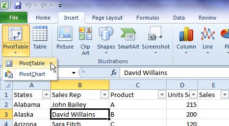
2. On the Insert tab, in the Tables group, click PivotTable and from the drop-down list select  PivotTable.

3. In the Create PivotTable dialog box, in the Choose the data that you want to analyze section, verify that Select a table or range is selected, and then in the Table/Range box, verify that the range of cells that you want to use is selected.

4. In the Choose where you want the PivotTable report to be placed section, select a location and click OK.

5. The PivotTable is displayed in a new worksheet if the default option is selected.

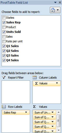
6. Use the PivotTable Field List pane to create the PivotTable.

• Drag the field names from the top to one of the four boxes at the bottom of the pane.

• Check the item at the top of the PivotTable Field List. Excel will automatically place the field into one of the four boxes at the bottom of the pane.

• Right-click a field name at the top of the PivotTable Field List and choose its location from the context menu.

7. Your PivotTable is now ready with summarized data.

Now that you’ve created a PivotTable report, you can format it, make modifications to the data and use it for analytical purposes.

Before you can manipulate the PivotTable to analyze the data in your worksheet, you should be familiar with the various components of the Pivot Table. Familiarize yourself with the common PivotTable terms used while working with the Excel feature.

Source Data: The data used to create a pivot table. It can be located within a worksheet or in an external database.
Item: It is an element that appears as a row or column header in a pivot table.
Column Labels : It is afield that displays data as categories or groups in a single column in the PivotTable. You can drag any item in the PivotTable Field List Task pane to the Column Labels list box to create a column label.
Row Labels: It is a field that displays data as categories or groups in a single row in the PivotTable. You can drag any item in the PivotTable Field List Task pane to the Row Labels list box to create a row label.
Grand Total: It is a field that displays the sum totals for all cells in a row or column.
Subtotals: It is a field that displays the subtotals for a category of cells in a row or column.
Values Area: It is the area in a PivotTable that contains the summary data.
Page Field: It is a field that can be filtered to display only the data you want to view in the PivotTable.

MORE PIVOT TABLE LEARNING

If you are keen to learn the basics of Pivot Tables including:

• How to setup a pivot table in Excel 2010
• How to setup a pivot table in Excel 2013
• How to filter a pivot table and chart; and
• Use Slices

You can give the “Learn Microsoft Excel Pivot Tables” course from Udemy a try. The course is packed with great training that will have you instantly replicating them at your workplace.